SUMIF vs SUMIFS in Excel: Why the Argument Order Bites
SUMIF puts the sum column last and SUMIFS puts it first. Swap the columns in SUMIF and Excel returns 0 with no error, so the order matters.

SUMIF and SUMIFS both add up values that meet a condition, and their names differ by one letter. The argument order is where they diverge, and getting it wrong doesn't always produce an error. Sometimes it just gives you a quiet zero, which is the worse outcome in a report.

SUMIF: the sum column goes last
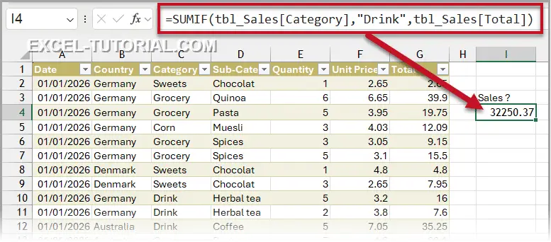
SUMIF takes three arguments in a fixed sequence: the column where you look for the condition, the condition itself, and the column to add, which sits in last position. To total the sales of the Drink category, the formula reads:
=SUMIF(tbl_Sales[Category],"Drink",tbl_Sales[Total])
Swap the columns and Excel stays silent
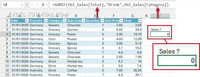
Now reverse the two column references, so the Total column is tested against "Drink" and the Category column is summed:

=SUMIF(tbl_Sales[Total],"Drink",tbl_Sales[Category])
Excel accepts this without any error message and returns 0. It is looking for the word "Drink" inside a column that holds only numbers, so nothing matches and nothing gets added. On a report with dozens of totals, a zero like this is easy to miss, especially when it sits in a cell that already looks plausible. That silence is the real hazard here, more than the wrong answer itself.
💡 Keep the rule in mind: with SUMIF, the column to add goes at the end. SUMIFS changes exactly that.

SUMIFS: the sum column moves to the front
In SUMIFS, the column to add moves to the first position. After it come pairs of "column to test, condition". The same calculation becomes:
=SUMIFS(tbl_Sales[Total],tbl_Sales[Category],"Drink")
The two functions compare like this:

- SUMIF: the column to test, the condition, then the column to add as the third and final argument.
- SUMIFS: the column to add first, then the pairs of column to test and condition.
Why the order differs
SUMIF is one of Excel's oldest functions, and it was built for a single condition. That design let the column to add sit at the end, and it is even optional. Under the same logic, the sum range can be left out when the condition column is the one you want to add.
SUMIFS arrived in Excel 2007, alongside COUNTIFS and AVERAGEIFS. It accepts up to 127 conditions, so Excel has no way to tell where the list of conditions ends. The only fixed position left for the column to add is the first one, which is why the order flips.
Changing SUMIF itself was never a realistic option, because that would break a very large number of existing workbooks. Both syntaxes therefore sit side by side in current versions. The same inversion shows up between AVERAGEIF and AVERAGEIFS, so anyone who learned one pair has probably tripped over the other.
The habit that prevents the error
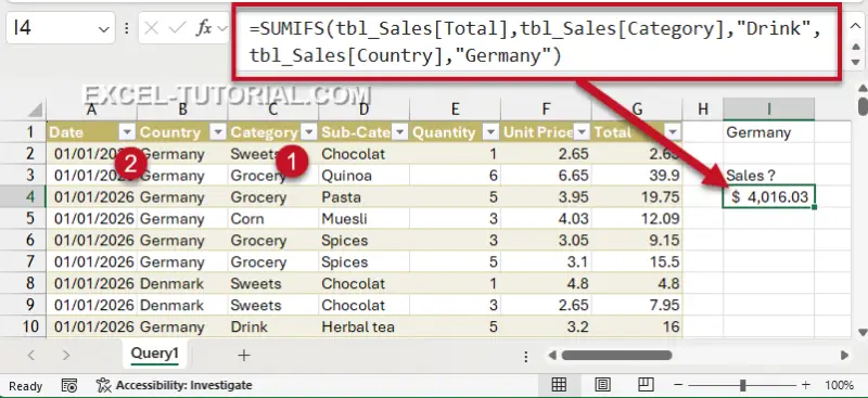
My suggestion is to standardise on SUMIFS, even when you only have one condition. You then carry a single syntax in your head, the same one that COUNTIFS and AVERAGEIFS follow. Adding a second condition is simply a matter of appending another pair at the end:
=SUMIFS(tbl_Sales[Total],tbl_Sales[Category],"Drink",tbl_Sales[Country],"Germany")
What to check in your own workbooks
If you maintain existing sheets, it's worth scanning for SUMIF formulas that return zero where you expect a value. A zero from a column that should contain totals is a good signal that the arguments were swapped. Converting those formulas to SUMIFS removes the ambiguity, and the new structure makes the sum column obvious at a glance.
That said, you don't need to rewrite everything in a hurry. Where SUMIF already works and is well understood by your team, leave it alone. The point is to stop the silent-zero failure from creeping into new work, and a consistent SUMIFS habit does that cheaply.


